Blog

Disclaimer
In the third article I wrote about this topic I said it was going to be the last one. I lied. The thing is that there is more to talk about this application, and you may well wonder why.
Fortunately, Juan Pablo Blanco (the one who came up with the app and one of its creators) read my posts and liked them.

We started exchanging ideas on Twitter about the algorithm, and more generally speaking, what this type of methodologies can be used for. We also discussed carrying out projects together. So much so, that we promised to keep in touch.

The encounter
We agreed to meet at “DATA Cafés”, a meetup organized by Cívico  y DATA Uruguay  The aim of these meetings is basically to share ideas in connection with open data.
This time the theme was how to create tools and projects involving data, for next election’s purposes. The activity was part of the Open Gov Week, with the aim of generating civic technology tools to find information, follow, and have a better understanding of the electoral process.

Several interesting ideas came up at the meeting. For instance:
• “Chose Legi”: an app to learn the last 30 laws passed at parliament. You are asked to vote, and next your vote is compared to that of current deputies and senators. It’s a good idea because I think everyone would be interested to know what legislators vote for, but even if it seems unbelievable, there is no easy access to that information in Uruguay.
• Beating fake-news with data. For instance: http://uycheck.com/
• Charge graphs: it is a timeline showing the positions held by each congressman/senator/minister/etc. throughout their life. The whole C.V. is exposed see their performance both the private sector and the government.
• Estate Affidavits: it is an analysis of representatives’ assets and income.
• Jingle analysis: applying text analytics techniques to political jingles
• Declaration of Principles: ask candidates running for the Legislative Power to state and sign their commitment to open up parliament, to facilitate access to information.
• Aquienvoto.uy 2.0: would give you advice on which candidate is closer to your ideology, rather than to other people’s. To this end, a new set of questions should be made to candidates, etc.
After the meeting, Juan Pablo, Rodrigo Conde (another of the developers of aquienvoto.uy) and I stayed discussing more in depth.

Model Change
Only days before, I had read a tweet where someone said they had changed the app’s algorithm

I told Juan Pablo about the new model, and so on. As I did in my first post with Kneighbors, I will now try to explain how the Logistic Regression algorithm works.
Logistic regression is among classification algorithms and, contrary to how linear regression works, it is used to predict discrete (non-continuous) data; it works both to predict binary results(0 or 1 , yes or no, sick or healthy, etc.) and to classify information into multiple classes.
For example, it can predict whether a person will have an adverse reaction to a drug, whether it will be cloudy, sunny, or rainy, among others. For the logistic regression the objective is not to predict a real number. As seen in the weather example, it is also important to note that the label does not have to be binary, but there must be a finite number of labels.
I didn’t ask the guys why they had changed the model, but I dare guess some reasons.

KNeighbors Defects
The above algorithm, known as the nearest neighbor, is very beautiful for its simplicity, so much so that anyone – even if they are no connected to I.T. – can rapidly understand how it works. I believe this is also one of its main flaws.
It is too trivial for some cases, in fact it does not learn anything, its machine learning component is very basic: all the computer has to do is remember. The machine “memorizes” the training data, and when we want to predict the label of a new example, we look for the closest example in the training data, and assume that it must belong to the same category.
The biggest problem with this algorithm is noise, which is when training information has been misclassified: if the nearest neighbor has been the wrong choice, then I a new event will be misclassified as well. To mitigate this problem the closest K is searched, and the “most frequent” label is chosen.
Determining that K, and the number of neighbors to consider, is quite an issue.
Let us analise a real-life example to understand it better. Imagine we want to predict who will vote for someone living in Arocena and Rivera, half a block from the Carrasco Lawn Tennis Club. I can ring the bell on their closest neighbor, and ask them who they are going to vote for. That neighbor may vote for the Broad Front (20.43 % of Carrasco’s people do) or for the Colorado Party (20.39 percent of that neighborhood vote for Batlle y Ordoñez’s Party). However, if instead of asking the nearest neighbor we take into account the 10 closest neighbors and we see which party the majority of those 10 vote for, the prediction will probably be the National Party because 48.9% of people living in Carrasco do so. Along the same lines, if we enlarge the number of nearest neighbors to 1.5M, the prediction will be a Broad Front voter, since the government’s party adhesion in Montevideo is 53.51%.
You see in that example that if we select a large K the result will be strongly influenced by the size of the classes. If in the training data we have many more voters for the Broad Front than any other, and we choose a big K, then the prediction will tend to be that one. That’s probably what happened to aquienvoto. The candidate with most votes was Talvi, and that’s why the prediction for many people was him.
Even if learning KNN is very quick, for all you have to do is memorize everything, and not much math is needed, the disadvantage is that if I have millions of examples to keep, they occupy too much memory. Another drawback is that every time I want to predict something, this may take a long time, since we would have to find the distance of the case we want to predict against all the ones I have. This is the toll to pay for not having overhead in pre-processing (however, there are better algorithms than mere strength for reach the closest K).
Moreover, we cannot tell how the process works or have an actual model to be used as an example to make a lineal regression.
After having presented what I consider the disadvantages of the earlier model, I will try to explain the new method, which is the most common method used in machine learning: logistic regression.

Logistic Regression
As we have already mentioned, logistic regression is somehow like lineal regression, but some of their crucial aspects are different. Lineal regression is used to predict a real number, in this case what we want to learn is how probable the occurrence of an event is. That is, we know that the dependent variable can have only a finite set of values (for example, running candidates). The problem with lineal regression is all the time you get predictions that don’t make sense, you can’t vote half for one candidate and half to another or be 1/3 ill. Someone might say that 0.5 may mean that there’s 50% chance that this person vote for a certain candidate, rather than half-candidate, but if we see a little bit further in a linear regression, values may be higher than 1 or lower than 0. This makes no sense in terms of probabilities.
What linear regression does, is finding the weight of each characteristic.
What we do is take each characteristic (each of the questions on the form) and calculate a weight for each of them which we will use to make predictions. Weights play the role of coefficients when we are doing a linear regression.
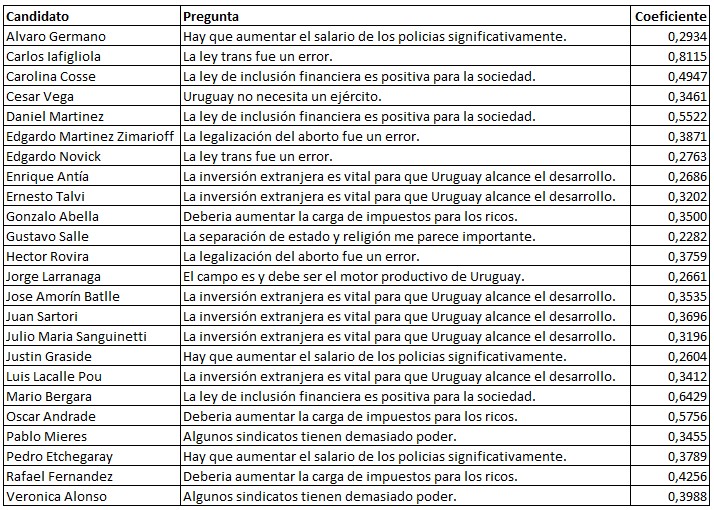
So basically, we have coefficients associated to each variable. We will add those coefficients, and multiply them by something and make a prediction. A positive weight implies that that variable is positively correlated with the output. For example, the statement “The trans law was a mistake” is positively correlated with voting for Carlos Lafigliol: the coefficient is 0.8115!
On the other hand, a negative weight shows that the variable is negatively mapped to the output. Consequently, the statement “The Army should play an active role in public safety” has a negative weight (-1,2188) in the case of candidate Hector Rovira. The correlation is negative. In other words: the more someone agrees with this statement, the lower the chances are that they vote for the retired colonel. It is not absolute, just a correlation.
Once the model is trained and the weights for each feature are awarded, a new set of features (answers to questionnaire questions) can be easily introduced, and the model delivers the probability associated with each label (i.e. the probability associated with voting for each candidate).
The good thing about this algorithm is that, while it may be slow to generate the model, once it is done, it is fast to classify, since it works regardless the dataset size used for training. Once we have the coefficients, it is basically a polynomial evaluation.
The other advantage that I consider even more important is that it yields insights (findings) on variables. Coefficients show how variables correlate to each labels. For example, in the following table we see which question is most related to each candidate:

Will logistic regression be the best algorithm to make these predictions? Stay tuned for the next article.

Héctor Cotelo  @CoteloHector

Consultor en Data Analytics & Information Management